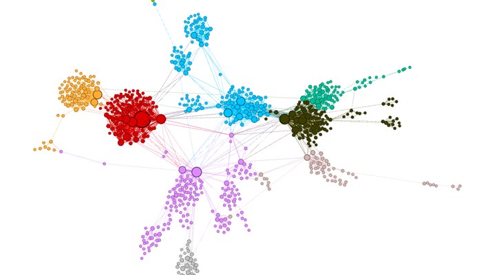
Understanding and Visualizing Word Embeddings with GloVe and Word2Vec

Word embeddings are like a secret sauce in natural language processing. They allow machines to understand and represent the meaning of words in a high-dimensional space. In this blog post, we’ll explore two popular word embedding techniques, GloVe and Word2Vec, and learn how to visualize them using Python. By the end of this post, you’ll be visualizing word embeddings in your own project using Python.

Preprocessing Text Data: Tokenization, Stopword Removal, and Stemming

Before diving into word embeddings, it’s crucial to preprocess the text data. This involves three key steps:

1. Tokenization: Breaking the text into individual words (tokens).
2. Stopword Removal: Removing common words like ‘the’, ‘and’, ‘is’, etc., that do not contribute much to the meaning.
3. Stemming: Reducing words to their root form, e.g., ‘running’ to ‘run’, to simplify the data.

Imagine your text data as a messy room. These preprocessing steps help clean and organize it, making it easier for the word embedding models to work with the data.

Step 1: Preprocess the Text

First, let’s start with preprocessing the text. You can clone the repo here. Text preprocessing typically involves tokenization, removal of stopwords, and stemming. Below is a Python function that takes raw text as input and returns preprocessed tokens:

import nltk
from nltk.corpus import stopwords
from nltk.stem import PorterStemmer
from nltk.tokenize import word_tokenize

nltk.download('punkt')
nltk.download('stopwords')

def preprocess_text(text):
    # Tokenize the text
    tokens = word_tokenize(text.lower())
    
    # Remove stopwords
    stop_words = set(stopwords.words('english'))
    filtered_tokens = [token for token in tokens if token.isalnum() and token not in stop_words]
    
    # Stemming
    stemmer = PorterStemmer()
    stemmed_tokens = [stemmer.stem(token) for token in filtered_tokens]
    
    return stemmed_tokens

GloVe and Word2Vec: Two Powerful Word Embedding Techniques

Global Vectors for Word Representation

GloVe, short for “Global Vectors,” is a word embedding technique that uses co-occurrence statistics from a large text corpus. It captures both global and local information by examining word pairs and their frequency in the corpus.

Think of GloVe like a treasure map. By examining the relationships between words in a text corpus, it uncovers hidden patterns and creates word embeddings that capture the meaning of each word.

Word2Vec: Continuous Bag-of-Words and Skip-gram Models

Word2Vec is another popular word embedding technique that comes in two flavors: Continuous Bag-of-Words (CBOW) and Skip-gram. CBOW predicts a target word based on its context, while Skip-gram predicts the context words given a target word.

Imagine Word2Vec as a jigsaw puzzle. It learns word embeddings by trying to fit words together based on their context, creating a high-dimensional representation that captures the meaning of each word.

Step 2: Train Word Embeddings

Next, we will train word embeddings using the GloVe and Word2Vec models. For GloVe, we load pre-trained embeddings into a dictionary. For Word2Vec, we train embeddings using the Gensim library:

import numpy as np
from gensim.models import Word2Vec

raw_text = """
I love machine learning. It is awesome!
Deep learning and natural language processing are very cool.
Artificial intelligence is the future.
"""

preprocessed_tokens = preprocess_text(raw_text)

# Load GloVe embeddings
glove_embeddings = {}
with open("/path/to/glove.6B.50d.txt", "r") as file:
    for line in file:
        values = line.split()
        word = values[0]
        vector = np.asarray(values[1:], dtype="float32")
        glove_embeddings[word] = vector

# Train Word2Vec embeddings
model = Word2Vec([preprocessed_tokens], min_count=1, vector_size=50, workers=4)

Visualizing Word Embeddings using t-SNE

t-SNE (t-distributed Stochastic Neighbor Embedding) is a dimensionality reduction technique that allows us to visualize high-dimensional data in a 2D space. In our case, we’ll use t-SNE to visualize the word embeddings generated by GloVe and Word2Vec models.

Picture t-SNE as a magnifying glass. It helps us zoom in on the high-dimensional word embeddings and visualize their relationships in a 2D space.

Step 3: Visualize Word Embeddings

For our final step, now that we have our word embeddings, let’s visualize them using t-SNE, a dimensionality reduction technique that helps us project high-dimensional data into a 2D space:

import matplotlib.pyplot as plt
from sklearn.manifold import TSNE

def visualize_embeddings(embeddings, words):
    tsne = TSNE(n_components=2, random_state=0, perplexity=len(words)-1)
    embedding_vectors = np.array([embeddings[word] for word in words])
    two_d_embeddings = tsne.fit_transform(embedding_vectors)

    plt.figure(figsize=(8, 8))
    for i, word in enumerate(words):
        x, y = two_d_embeddings[i, :]
        plt.scatter(x, y)
        plt.annotate(word, (x, y), xytext=(5, 2), textcoords="offset points", ha="right", va="bottom")
    plt.show()

# For GloVe
glove_words = [word for word in preprocessed_tokens if word in glove_embeddings]
visualize_embeddings(glove_embeddings, glove_words)

# For Word2Vec
word2vec_words = model.wv.index_to_key
visualize_embeddings(model.wv, word2vec_words)

Putting It All Together: Visualizing GloVe and Word2Vec Embeddings

This code defines a function called visualize_embeddings that takes an embeddings dictionary and a list of words as input. It uses t-SNE to project the embeddings onto a 2D space and plots them using Matplotlib. To visualize the embeddings for GloVe and Word2Vec, we call the function with the respective embeddings and words.

Running this code will display two plots, one for GloVe and one for Word2Vec, showing the 2D representation of the word embeddings. The words are labeled, and you can see how words with similar meanings are grouped together in the 2D space. This visualization helps us understand the relationships between words and how the embeddings capture the meaning of the words in the text.

We’ve walked through the process of preprocessing text using tokenization, stopword removal, and stemming, training word embeddings with GloVe and Word2Vec, and visualizing the embeddings using t-SNE. Understanding and visualizing word embeddings is crucial in natural language processing tasks and can provide valuable insights into your text data.

Finally, to follow along with me while I complete the #100DaysofML Challenge and build machine learning projects of your own, subscribe for updates.

---